This post summarizes research by the Center for Cryptoeconomics. See the full report here. This research was funded by cyber.Fund. The opinions expressed in this post are solely those of the authors Juan Beccuti, Thunj Chantramonklasri, Matthias Hafner, and Nicolas Oderbolz. We thank @artofkot, @kkulk , @PaulYa5hin and @thelazyliz for their invaluable support, comments and reviews.
TL;DR
With the goal of contributing to the study of how changes in Ethereum’s issuance curve affect the staking decisions of different categories of stakers and, consequently, the degree of decentralization in the staking market, we develop a game-theoretic model of the Ethereum staking market and use it to conduct a comparative analysis of different issuance schedules. We discuss the results of this analysis in the context of the available empiricial literature, as well as our own preliminary estimates of staking supply elasticities. In addition to contributing to the debate on reducing protocol issuance, we expect that the model can serve as a basis for further extensions, providing a flexible framework for analyzing staking dynamics under different protocol changes.
Existing empirical research, as well as our own estimates using an Instrumental Variable (IV) approach, tends to suggests that solo stakers may be more sensitive to changes in staking yields than other staking categories.
The game-theoretic model presented below shows that a staker’s equilibrium staking supply is determined by their staking costs and revenues, as well as the strategic behavior of other market participants. Our results suggest that later competitive market forces may be important in explaining why solo stakers are more sensitive to changes in staking yields. Other staking categories benefit from additional revenue streams, such as superior MEV access and DeFi yields, which makes them less responsive to changes in consensus rewards. Given Ethereum’s downward-sloping issuance schedule, strategic solo stakers internalize these competitive pressures, rendering them more sensitive to changes in consensus yields.
By comparing the equilibria of our model under the current issuance schedule with those of a proposed alternative, we find that reducing issuance could exacerbate this effect. While a change in the issuance schedule in our model is associated with a reduction in the supply of staked ETH across all staking categories, it is also associated with a reduction in the market share of solo stakers and an increase in the market share of liquid staking solutions.
Additionally, our model predicts that solo staking becomes less profitable than other staking methods. While outside of the scope of our model, this could undermine the long-term viability of solo staking and accelerate the exit of solo stakers from the market in favor of alternative solutions, such as decentralized staking service providers and liquid staking.
Motivation
As the volume of ETH staked within Ethereum’s Proof-of-Stake (PoS) protocol has grown significantly over the past few years, discussions around the long-term sustainability of the current issuance schedule have become prominent. Central to this debate is the trade-off between the efficient use of validator infrastructure, issuance-driven inflation, and economic security.
A reduction in the consensus issuance schedule has been argued to be important in avoiding an end-game scenario in which most of the circulating supply of ETH is staked (see for example Elowsson (2024) and Schwarz-Schilling (2024)). Such an outcome would mean that the supply of staked ETH far exceeds the necessary threshold for economic security, resulting in unnecessary inflationary pressure and inefficient allocation of validator resources. In addition, there are concerns about the potential systemic risks posed by the proliferation of liquid staking tokens and their potential to replace ETH as the de facto currency in the ecosystem. These considerations suggest that it may be prudent to revise the issuance schedule to effectively reduce the incentives for staking.
Conversely, a reduction in staking rewards may disproportionately affect the profitability of relatively expensive decentralized staking solutions compared to centralized solutions, and thus may result in less decentralization. In particular, solo stakers, who already represent a small segment of the total validator population, may be disproportionately driven out of the market.
In what follows, we aim to test the validity of this argument by examining how different staking methods, and in particular solo stakers, may be affected differently by changes to Ethereum’s consensus issuance policy. Specifically, we focus on answering two key research questions:
- How do different types of stakers respond to shifts in the issuance schedule?
- How might these changes impact the decentralization of the Ethereum staking ecosystem?
Methodological Approach
To address these research questions, we employ the following methodological approaches, the results of which we highlight in this post:
- Empirical Estimation: We use an Instrumental Variable approach to estimate how changes in staking rewards affect the supply of staked ETH across these different staking categories.
- Game Theoretic Model: Guided by the empirical results, we develop a game-theoretic model of the Ethereum staking market in which staking agents of different types determine their staking supply based on the revenue streams and cost structures associated with different staking methods. The goal is to construct a modeling framework that links individual staking decisions to the aggregate staking supply in the Ethereum staking market.
- Simulation and Comparative Analysis: By simulating this game-theoretic model under various parameter configurations, we seek to understand how individual cost structures and revenue streams influence equilibrium outcomes in the aggregate staking market. In addition, we calibrate the model to specific parameter settings and evaluate how changes in Ethereum’s issuance schedule could affect staking market outcomes, in particular the market shares of different staking categories.
Estimation of Staking Supply Elasticity
Methodology
We estimate the sensitivity of staking supply to changes in staking rewards across different staker types. To address endogeneity concerns, we employ an Instrumental Variable (IV) approach. Endogeneity is an issue in this context, since any combination of staking yields and staking supply observed at a given point in time is in theory a result of a market equilibrium, where the supply and demand for staking meet. Changes in this market equilibrium can arise from both shifts in the supply curve and shifts in the demand curve, creating endogeneity in any simple estimate of the correlation between staking yields and staking supply. The purpose of this estimation approach is thus to identify instruments that shift the demand curve for staked ETH without simultaneously affecting the factors determining the supply curve. Using such instruments allows us to isolate the shape of the supply curve, at least at a local equilibrium point.
For the estimation of the yield elasticities of supply for different staking categories, we propose the use of gas fees as a robust instrument. Gas fees may represent a valid instrument in this context, because they directly influence staking rewards but remain exogenous to the determinants of staking supply, as they are driven by external factors such as network activity, DeFi transactions, and NFT trading. Leveraging the natural fluctuations and publicly available gas fee data, we conduct a two-stage least squares (2SLS) analysis using daily-level data, with rewards and amount staked denominated in USD. A detailed description of the estimation approach and the corresponding results is provided here.
Results
Importantly, the approach yields estimations of the yield elasticities of supply that suggest that the staking supply of solo stakers is more sensitive to changes in staking yields compared to the staking supply of the overall population of stakers. The elasticity of staking supply to staking rewards is estimated at 1.184 for solo stakers and 1.078 for all stakers. Both estimates are statistically significant at the 1% level. These results are generally consistent with the findings of Eloranta and Helminen (2025), whose estimations similarly suggest that solo stakers are more sensitive to changes in the staking yield than the overall population of stakers.
Table 1: 2SLS estimates with gas fees used as an instrument for staking rewards| Solo Staking | All Staking Types | |||
|---|---|---|---|---|
| (1) Log Amount Staked (USD) | (2) Log Amount Staked (USD) | (3) Log Amount Staked (USD) | (4) Log Amount Staked (USD) | |
| Log Rewards (USD)t | 1.184*** (0.073) | 1.078*** (0.035) | ||
| Log Rewards (USD)t−1 | 1.176*** (0.074) | 1.075*** (0.036) | ||
| Constant | 6.774** (0.877) | 6.868*** (0.888) | 7.739*** (0.543) | 7.786*** (0.556) |
| Observations | 622 | 621 | 622 | 621 |
| R-squared | 0.128 | 0.101 | 0.858 | 0.851 |
| Note: The coefficients reported in this table can be interpreted as the yield elasticities of staking supply. The coefficients report the estimated percentage increase in the amount of ETH staked (denominated in USD) that is associated with a 1% increase in the USD value of staking rewards, either in the same period or a one-week lag. Columns 1 and 2 report the results estimated on the sample of solo stakers. Columns 3 and 4 report results estimated on the full sample of staking. Robust standard errors are reported in parentheses. | ||||
| *** p<0.01, ** p<0.05, * p<0.1 |
Game-theoretic Model
To further understand what drives staking supply elasticities, we develop a game-theoretic framework that allows us to model the strategic staking decisions of different staking market participants as a function of the Ethereum issuance schedule, other external revenue sources, and the cost of staking.
Agent Types
We propose a game-theoretic model of a segmented staking market, where ETH holders are differentiated based on their preferences and/or level of technical sophistication, which in turn determines how they will stake. Specifically, three distinct types of ETH holders are considered:
Each category comprises a fixed number of stakers, denoted as N_rNr, N_tNt, and N_{ss}Nss for Retailers, Techies, and Experts (or Solo Stakers), respectively. To ensure tractability, within-group homogeneity is assumed.
Segmented Staking Market
In addition, the model incorporates several staking methods that differ in both the costs they impose on the ETH holder and the revenue streams they provide. These methods include solo staking, staking through a centralized service provider (cSSP), such as a centralized exchange or a professional direct staking delegation company like Kiln, and staking through a decentralized service provider (dSSP) that provides additional DeFi yields through an LST, such as Lido. We do not model restaking explicitly.
Each type of ETH holder has different staking options based on their level of expertise. In principle, Retailers stake exclusively through a centralized staking service provider (cSSP); Techies choose between a cSSP and a decentralized provider (dSSP); and Experts can access the full range of options, including solo staking.
However, we model revenues, cost and preferences that results in a segmented staking market. That is, each ETH holder selects a single staking method or stays out, and does not diversify across options. Specifically:
- Retailers either stake with a cSSP or abstain, reflecting a preference for ease of use and limited technical capacity.
- Techies prefer dSSPs over cSSPs because they receive higher returns from LSTs. That is, we model revenue and cost functions such that Techies’ profits are larger than Retailers’s ones.
- Experts are assumed to exclusively choose to solo stake—despite potentially lower profits—due to an intrinsic (but unmodeled) utility derived from contributing to decentralization. As a consequence, Experts solo stake or leave the staking market.
Note that segmented staking markets are also considered in other studies, such as Kotelskiy et al. (2024). Also note that we do not model the staking decision as a portfolio allocation problem. Instead, each ETH holder allocates their entire stake to the option that yields the highest utility for their type. This framework emphasizes clear segmentation rather than hybrid strategies. An alternative approach could involve portfolio management. In that case, the model presented below would require modifications to avoid corner solutions—for example, by explicitly incorporating Experts’ intrinsic preferences for decentralization.
Staking Revenues
Depending on the staking option they choose, ETH holders may receive revenues from three different sources: 1) consensus layer revenue, 2) MEV revenue, and 3) additional DeFi yield.
The first is consensus layer revenue, determined by the protocol’s issuance schedule. The annual consensus yield provided to an ETH holder ii when staking is denoted as y_i(D)yi(D). Under the current issuance schedule, the annual consensus yield is given by
where DD represents the total amount of ETH staked in the protocol. In later sections, we will compare model outcomes under the current issuance schedule y_i(D)yi(D) to those under an alternative specification y_i'(D)y′i(D).
The second revenue source is MEV revenue. Validators selected as proposers in block production can extract additional revenue from structuring transactions, referred to in the following as MEV revenue. Letting N = D/32N=D/32 denote the total number of validators, the probability that an ETH holder controlling d_i/32di/32 validators is chosen as a proposer is d_i/Ddi/D. Conversely, if a staker joins a staking pool (i.e. stakes with an intermediary), proposers may share MEV revenues with others in the pool. The probability that any validator in the pool is selected as a proposer is d_{pool}/Ddpool/D, and a validator with stake d_idi receives a share of d_i/d_{pool}di/dpool. Thus, the expected MEV revenue for a staker in a pool remains the same as for a solo staker. In both cases the expected annual MEV revenue y_vyv for an ETH holder is theoretically given by
The third source of revenue is additional DeFi yield. ETH holders utilizing a dSSP may earn additional yields by reinvesting the LST they receive. The annual yield from this source of revenue is simply defined as y_dyd.
Staking Costs
From the perspective of the ETH holder, staking is associated with different costs. In the present model, the cost function faced by an ETH holder is allowed to differ for each staking solution. We define a cost function that include fixed costs and non-linear variable costs
Later, we calibrate the model looking for the set of parameters that gives a similar distribution of staking supply than the one observed in the market at the moment of this study. We also assume that the costs functions are such that there are interior solutions. This assumption is standard in models where agents face no binding constraints on their choices, such as budget constraints.
Furthermore, ETH holders staking through an intermediary incur fees, which are modeled as a tax on revenues and as such treated separately from the cost functions. The cSSP fee rate is denoted as f_cfc, and the dSSP fee rate as f_dfd, both of which are assumed to be exogenous in the baseline model. As such, fees are simply assumed to be fixed and not determined by the strategic behavior of the staking service providers in the market. Subsequent extensions will relax this assumption and to some extent allow fees to be determined as a function of the profit maximization problem of the staking service providers in the model.
Staking Decisions
Under the assumption of a constant ETH price, thus isolating staking decisions from price volatility and inflation effects, each staker maximizes expected annual profit.
Given the deposits of other stakers \{d_{ss},d_r,d_t\}{dss,dr,dt}, a representative Expert chooses a deposit \hat{d}_{ss}\geq 0^dss≥0 to maximize
with
and such that their profits are not negative (negative profits implies no staking).
Let P_{ss}(D)Pss(D) denote the probability that a staker with deposit \hat{d}_{ss}^dss becomes a proposer. We model this probability as the ratio of the staker’s deposits to the total deposits, as indicated in the denominator. However, a more accurate representation would model this as the ratio of the number of validators controlled by the staker to the total number of validators. This would require a step function that increments with every 32 ETH, corresponding to the validator activation threshold. For tractability, we instead model P_{ss}Pss as a continuous function of \hat{d}_{ss}^dss, which simplifies the analysis.
\hat{d}_{ss}^*^d∗ss denotes the optimal choice of the maximization problem. Due to homogeneity within each staker type category, all Experts must choose the same deposit level in equilibrium. That is, in equilibrium, the individual optimal choice \hat{d}_{ss}^*^d∗ss satisfies \hat{d}_{ss}^* = d_{ss}^d∗ss=dss.
Similarly, each Techie chooses a deposit \hat{d}_{t}\geq 0^dt≥0 to maximize
with
Homogeneity again implies \hat{d}_t^*=d_t^d∗t=dt. Notice that this type of staker pays a fee f_dfd and enjoys of DeFi yields y_dyd.
Retailers choose a deposit \hat{d}_{r}\geq 0^dr≥0 to maximize
with
Again, homogeneity implies \hat{d}_r^*=d_r^d∗r=dr.
Depending on their type, these ETH holders make strategic decisions about how much ETH to stake. In effect, they choose their profit-maximizing supply of staked ETH taking into account their costs and fees to pay, and their expected revenues while anticipating the staking behavior of the other agents. The full paper provides a detailed description of the model and the derivation of the resulting Nash equilibrium.
These above staking decisions define the strategic behavior of different agent types in the baseline model. However, real-world staking is subject to additional complexities, which we now introduce as model extensions.
Model Extensions
We extend the baseline model in several key ways, adding important details to the characteristics of staking agents as well as the intermediary market (please refer to the full report for a formal description of these extensions):
- Variability in MEV rewards for solo stakers: We assume that the staking type Expert is risk-averse and experiences a disutility from the variance in MEV revenues. The profit maximization problem for the other staker types remains unchanged. This formulation accounts for the fact that solo stakers may require several years to propose a block with high MEV, unlike other stakers in a pool who can benefit from smoothing MEV revenues over time.
- Non-strategic staker type: We divide the Retailer category into two subgroups: (1) institutions and (2) inattentive retail investors. The latter group is assumed to be unresponsive to changes in the issuance yield, meaning they do not behave strategically. This behavior could stem from their inelasticity, but a more realistic interpretation is that they are inattentive agents or that their profit-maximizing decisions result in a corner solution (staking either all or none). The primary purpose of incorporating this type of agent into the model is to assess how their presence influences the staking behavior of other types, particularly solo stakers.
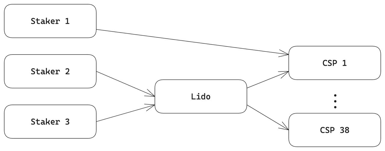
- Intermediary SSPs with market power: Finally, we add complexity to the intermediary market for staking providers by incorporating intermediary dSSPs with market power. In the baseline model, it is assumed that staking fees are fixed and as such that dSSPs operate under perfect competition and that they themselves provide the staking service. A more realistic approach would model dSSPs as intermediaries or middleware between stakers and centralized staking service providers (cSSPs). For example, when an ETH holder decides to stake with Lido, the stake is managed through a cSSP. Lido itself does not directly provide the staking service; instead, it facilitates the connection between the ETH holder and the cSSP. In this arrangement, the ETH holder benefits from Lido by receiving a derivative representing their stake. The following figure illustrates this setup in a simplified form.
Results
To assess how different issuance schedules impact equilibrium staking decisions, we compare staking outcomes under two alternative issuance rules. The first issuance schedule corresponds to the one currently implemented by the Ethereum protocol:
where DD represents the staking deposit level. The second issuance schedule follows one of the alternative proposals presented by Elowsson (2024):
where k=2^{-25}k=2−25 and DD again represents the total amount of ETH staked.
These schedules might influence staking incentives differently. Before comparing the equilibrium staking decisions, we first conduct numerical simulations to better understand the forces behind the impact of transitioning from y_i(D)yi(D) to y'_i(D)y′i(D).
Numerical Simulations
We run extensive simulations of the baseline model, randomly varying all parameters across 10 million runs. These simulations provide insight into how different parameters influence equilibrium adjustments when moving from y_i(D)yi(D) to y'_i(D)y′i(D).
Our key findings are as follows:
- Observation 1: Higher marginal costs lead to smaller adjustments in the equilibrium staking supply when transitioning from y_i(D)yi(D) to y'_i(D)y′i(D). This effect is illustrated in Figures 2a - 2c, using solo staking as an example.
- Observation 2: The presence of additional MEV revenues or DeFi yields dampens stakers’ responses to changes in the issuance schedule. Figures 2d and 2e illustrate this effect using staking via dSSP as an example.
- Observation 3: The sensitivity of different agent types to changes in the issuance schedule is interdependent. For instance, when Techies become less sensitive to issuance schedule changes—such as when additional DeFi yields are high—the sensitivity of Experts to a change in the issuance schedule increases. Figures 2f illustrates this effect.
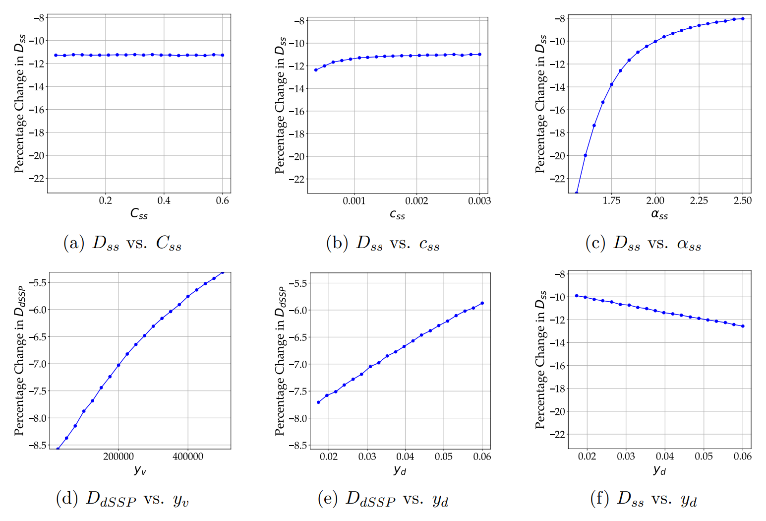
Note: The plots display the binned average percentage change in the total staking supply of different staking methods when transitioning from y_i(D)yi(D) to y'_i(D)y′i(D), categorized by different levels of model parameters. The number of bins is set to 20.
The simulations provide preliminary insights, but a structured comparison of equilibrium outcomes under the different issuance schedules is necessary. We now move to a comparative analysis that incorporates additional model refinements.
Model Calibration
We calibrate the model with specific parameters and compare Nash equilibria under two issuance schedules. Given the number of parameters to be calibrated, we find that estimating model parameters based on a method of simulated moments, i.e., algorithmically setting parameters to minimize the distance between simulated and observed market shares, does not provide a stable best fit. In other words, we find that a variety of possible parameter combinations can yield simulated market shares that are consistent with the observed data (see full report for more details).
As a second best approach, we propose parameter settings which are consistent with our qualitative understanding of the Ethereum staking market and that in the baseline model achieve a close fit to the observed market shares of the different staking types reported in Table 2. To shape our qualitative understanding, we conducted a survey for solo stakers on the Reddit forum r/ethstaker.
Table 2: Reference staking distribution used in parameter calibration| Staking Method | M ETH | % |
|---|---|---|
| dSSP | 18 | 54.1% |
| cSSP | 14.4 | 44.6% |
| Solo Staking | 0.9 | 2.7% |
| TOTAL | 34.2 |
Note: The estimated number of validators is based on a simplification of the categorization reported by Kotelskiy et al. (2024) and is calculated as the amount of staked ETH divided by 32. We categorize DSMs, LRTs, Whales, and Unidentified as dSSPs. Meanwhile, cSSPs consist of CSPs and CeXs.
Importantly, we assume solo staking incurs fixed costs, while staking via a dSSP or cSSP does not:
Contrary to staking through an intermediary, solo staking requires an individual to set up an Ethereum node with a running consensus and execution client. To do this, solo stakers can purchase dedicated hardware, subscribe to a cloud computing service, or use existing hardware. The costs associated with each of these options vary substantially. To further complicate matters, a range of hardware specifications can be used to run a node, each with varying costs. To date, the literature has made highly simplifying assumptions about the hardware costs of solo validators. In particular, both pa7x1 (2024) and Kotelskiy et al. (2024) assume that a solo staker factors in 1000 USD to initially purchase the necessary hardware, which they amortize over a period of 5 years. The anecdotal evidence collected from the survey on r/ethstaker generally supports this assumption but also reveals substantial variation owing to the fact that some stakers use existing hardware and do not purchase dedicated hardware for staking.
Similar to hardware costs, we assume costs for energy and internet to be fixed, since they are a fundamental requirement to running an Ethereum node but do not scale when adding additional validators to a node. Again, pa7x1 (2024) and Kotelskiy et al. (2024) assume around 1.4 to 2 USD in energy costs per week and around 0 to 12 USD per week for internet costs. These assumptions are generally supported by the anecdotal evidence from the r/ethstaker survey. However, there is likely substantial variation, since it is difficult to assume that hobbyist solo stakers would explicitly monitor and base their staking decisions on the internet and energy consumption of their solo staking setup.
Taken together, we assume fixed costs of \approx 1'000 \$/year≈1′000$/year. This includes hardware which is usually assumed to be amortized in 55 years (200-400200−400 \$/year$/year), high-speed and stable internet connection (5050 \$/month$/month), and additional electricity expenditures (100100 \$/year$/year). Denoting this cost in terms of ETH, at a price of ETH in USD of 2’400 USD, we obtain a parameter setting of C_{ss} = 0.4Css=0.4. Again, we assume that staking through an intermediary does not create any fixed costs from the perspective of the ETH holder. Thus, we set C_{r} = 0Cr=0 and C_{r} = 0Cr=0.
We further assume
The literature is much sparser on the variable costs of the various staking methods. As a result, we rely primarily on anecdotal evidence and simplifying assumptions. We argue that imposing the above c